In lesson 4 we looked at setting up a digital input to read a push button press. The polling implementation used is rather crude and not ideal in a real embedded system which interacts with many devices. The solution to this problem is interrupts, which allows the hardware to signal to the software that the button has been pressed. The implementation of interrupts is dependent on the architecture so in this lesson, we will dive in to the architecture of the MSP430. This will also prove to be extremely useful when debugging with mspdebug. When you compile the code, gcc automatically links against libraries which perform all the architecture and device dependent initialization required before you even get to ‘main’. Learning about these concepts are necessary to really understand how interrupts work and how they are implemented.
ELF object files and code sections
We are going to start this tutorial with some high level theory about object files. As we briefly discussed in earlier lessons, an object file is the compiled output of gcc, stored in ELF (Executable and Linkable Format). The ELF format defines the structure of the file, specifically the headers which describe the actual binary content (compiled code) of the file. The structure of the ELF file is interesting to read about, so if you are interested you can find more information here. For the purposes of this lesson, the important aspect of the object file is the concept of sections. Sections are groupings of a certain types of data which are stored in the object file and then transferred to the device flash when it is programmed. The type of section and all its attributes are stored in the section header (defined by the ELF format), and a pointer to where the section data is stored in the file. Section types can vary by architecture, compiler etc, so it is impossible to go through all of them, but there are a few which are almost always present:
- .data: where initialized read/write data is stored, for example a global or static variable with an non-zero initialized value i.e. int foo = 10; (NOTE: As Joel has pointed out in the comments below, MSPGCC places variables initialized to zero in the data section as well)
- .bss: where uninitialized read/write data is stored, for example, a global or static variable which is not initialized or initialized to zero. This section does not actually contain any data, only a pointer to the beginning of the section and the size. It must be initialized by the start-up code. At the application level, we can assume that statically defined variables are initialized to zero, but on bare-metal embedded systems this is not the case (note: we are on a bare metal system but gcc includes a library which does this initialization for us; this is not always the case).
- .stack: section which defines the stack. On the MSP430, the stack size is not defined, only a pointer to the top of the stack is included in this section. The top of stack is always the top of RAM, so the size of the stack depends on the amount of RAM in the device and how much data is being used by the rest of the program
- .const/.rodata: section where read only data exists. Stored on the flash on the MSP430. May include variables defined as ‘const’ and string literals.
- .text: section where the code is stored. Typically code is always read-only and therefore stored in flash, although on more complex systems, code has to be copied to RAM to run, therefore it can be modified
These are really the important sections that you need to know about in order to understand how the code organized after it is compiled. There are other sections which are added by the compiler and linker for optimization, relocation, debugging etc.. As you already know from the previous lessons, the size of RAM and flash differ from device to device. This means that the exact size and location of these sections cannot be hard-coded in the compiler. To account for this, the linker uses linker scripts to map the sections to physical addresses on the device.
Linker scripts
The linker script defines the memory map of the device with respect to the compiled code sections. It is required because the linker needs to know where in memory locate each of the sections of code based on the type of section and its specific attributes. For example, the linker needs to know to locate read/write data in RAM rather than in the flash memory address space. Sometimes linker scripts are modified by the developer to add custom sections for very specific purposes, but more often than not, the default linker script provided by the device manufacturer is sufficient for most all applications. Writing linker scripts is beyond the scope of this course, but we will explore the basics as it applies to this lesson. The linker script for the MSP430G2553 is located at
/opt/msp430-toolchain/msp430-none-elf/lib/430/msp430g2553.ld
Open the file in your text editor of choice. The first two lines of the script (past the comments) define the architecture and the entry point, _start. The symbol _start is the default entry point for gcc, and is included as part of the built-in libraries which we compiled when building the toolchain. When the device powers on or comes out of reset, it will jump to the address of this function.
Next you can see the ‘MEMORY’ tag which begins a table of the regions in memory, including their starting address and length. Most of these components we have already touched on. This table is really just a more detailed breakdown of the memory map introduced in lesson 3. The interrupt vector table will be covered in the next lesson, but if you recall from earlier lessons, it is just a table of functions. Scrolling down you can see the ‘SECTION’ tag which marks the beginning of the script which defines the sections. Skip past the interrupt vectors to the .rodata section. The .rodata section includes all the code compiled in .rodata and .const sections. There are two keywords which are used fairly often in this script, ‘KEEP’ and ‘PROVIDE’. ‘KEEP’ tell the linker to add the symbol in a section even if they are not used. Symbols are the human readable name for a function, variable etc… The symbol to address mapping, as well as the type of symbol and its attributes, is stored in the symbol table. It is used by the linker to resolve addresses while linking code. The linker may clean up unused symbols and code in order to reduce the size of the output. The keyword ‘PROVIDE’ tells the linker to define the symbol, but will only leave it in the symbol table if it used. In the case of .rodata, the symbols exported are all part of the initialization code, and are exported probably because they are required by the libraries. At the end of the .rodata section definition, which ends with a curly brace (“}”) , you can see that is mapped to a region using the greater than operator (“} > ROM”). This means that the .rodata section is to be placed in the ROM region of the memory map.
The .text section is defined next, which is also placed in ROM and provides both the _start symbol and etext/_etext/__etext (all the same symbol unless overloaded). The etext symbol marks the end of the text section. Why would you need this information? Well, for example, like the TLV section that we learned about in lesson 4, we may want to calculate the checksum of the .text section as well. Since we know that _start defines the beginning of the section and etext the end, we can calculate the size and hence the checksum (particularly useful for validating software upgrades in the field). Similarly, in more advanced systems where code should run from RAM for speed, it almost always the case that code is copied from its non-volatile source to RAM, and using these symbols makes this possible. To use the symbols, you must define them as extern in your source code.
Next is the .data section which is stored in ROM, but linked for RAM. This is because as we learned before, the .data section contains initialized variables which are read/write. So on a power up, the values have to be initialized correctly, hence stored in ROM, but linked for use in RAM. This means that although they are initially stored in flash, any code that accesses one of these symbols will be linked to its address in RAM. So how does the data end up in RAM? There is a function in the start-up code which copies the initialized data from ROM to RAM using the symbols provided just below: __romdatastart and __romdatacopysize which are assigned the address of the data in ROM and the size of .data in ROM respectively. The .data section also provide symbols which define the start and end of the the section in RAM: __datastart and __dataend / edata.
The next section in RAM is the .bss. The linker scripts provides the symbols __bssstart, __bssend and __bsssize which are used by the start-up code to zero out the portion of memory. Remember, this section does not actually contain any data. The reason for this is because it can drastically decrease the size of the executable / binary. Imagine on a device that supports Ethernet, you are creating a ring buffer for storing Ethernet frames. Each frame must be 1518 bytes and the ring has 10 elements. That’s 15800 bytes of zeros that would be in your image, which would then have to be flashed to the device. Its not the end of the world, but writing to flash is [relatively] slow, so it can make a difference.
The .noinit section is not used unless data is specifically put there either by directives in assembly or gcc attribute flags in C. Variables in the .noinit section are not initialized at start-up. It could be used for logging and debugging purposes. For example, your code is running and hits some critical error. The only option is to reboot. The error log can be written to a variable in the .noinit section and then when the device resets, the error log will still be there for some recovery code to identify and handle appropriately.
Finally the .stack section, which occupies whatever is left of RAM. At the top of the stack, a symbol __stack is provided which is copied to the stack pointer (explained in the next section) by the initialization code. Notice the stack is not a fixed size. If all the other sections in RAM only leave 2 bytes for the stack section, the compiler won’t complain. It will happily load your code, start running, and by the time one function call is made, or one word (16 bits) is allocated to the stack, you’ve blown the stack. Blowing the stack is a common problem and one that is very hard to identify. The repercussions are unpredictable, and the device may not even crash, it might just start corrupting data. Many operating systems provide stack checking and will at least notify you that you blew the stack. Later in the lesson I will show you how to determine how much stack if left once your code is compiled.
The rest of the linker script is for build and debugging information. Later in the lesson, we will see exactly the symbols defined in the linker script come into play on the MSP430.
CPU registers
Every CPU has a set of registers that can be used to load, store and manipulate data. As we discussed in previous lessons, registers are extremely fast memory. They are also the only way the CPU can perform calculations. For example, if you want to add two numbers both stored in RAM, the CPU cannot simply access the data and load it into the arithmetic logic unit (ALU – the part of the CPU that performs arithmetic operations). Each of the values (or a pointer to them) must be first loaded into registers and then the add operation can be invoked. When you add two variables in C, the compiler takes care of this for you in the most efficient way. Registers have specifically defined purposes as well, so not all registers would be used for the example above. The following diagram from the family reference manual shows the CPU registers in the MSP430.
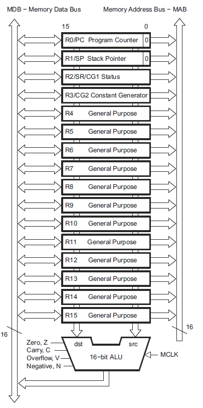
CPU Registers – from section 3.1 of SLAU144
To better understand this diagram, lets take a look at the purpose and use of each of these registers.
- program counter: contains the address of the current instruction. After each operation is completed, the program counter is incremented and the instruction at this address is read into the CPU and executed. The program counter on the MSP430 is register R0
- stack pointer: points to the address where the last value pushed on the stack is stored
- status register: a register that consists of a set of status fields such as carry, zero, overflow, negative, etc..
- constant generator: generate 6 predefined commonly used constant values for efficiency
- general purpose registers: used for arithmetic as above, passing arguments to functions etc…
At this point it is important to understand that if you were writing in assembly, other than the program counter, stack pointer, constant generator and status register, any of the other registers could be used at your discretion. However, writing complex programs put the onus on the developer to remember which register stored what value, and there would only be a finite number of values that could be held in registers at a time depending on the number of registers in the device. This is where high level languages come in and take advantage of the stack. Sure you could use the stack in assembly as well, but you would be effectively implementing the compiler yourself, and the compiler is [almost] always more efficient. The stack is an extremely important and often neglected topic. We learn about its use in more detail in the next section.
As for the general purpose registers, these are up for grabs in the compiler implementation. If I wrote a compiler, I could choose any of the general purpose registers to use for passing arguments. Then the next person could come along and choose a different set of registers for passing arguments. If code compiled by one compiler was linked with code compiled by the other, they would not correlate and it would not work. This is why device manufacturers release a specification called an Application Binary Interface, or ABI. This document defines how all of the registers should be used by the compiler, so that code compiled with different compilers that follow the standard can all play nice together.
The MSP430 ABI
The MSP430 ABI is located here. The specification covers topics such as data types, function calling conventions, data allocation, code allocation, etc.. It is a good document to read through for your own knowledge, and since it is defined for the architecture, all MSP430s will follow the same conventions. The information is extremely useful for debugging purposes, because you will be able to trace through the code and understand at the assembly level what the processor is doing. We will not go into depth on the actually assembly language (it is documented in the family reference manual if you are interested) because I want to keep these tutorials as generic as possible so it can be applied to any device. That being said, any time you do low level debugging, you will want to understand at least the basics of the ABI of the architecture you are working with.
At this time it is important to cover the topic of the stack. The stack typically accessed using ‘push’ and ‘pop’ instructions, that it is push some data onto the stack, and then pop it off. A hardware stack is pretty much identical in terms of functionality to a software stack. However, in the case of a hardware stack, the way it is used is defined by the ABI. Often, as is the case with the MSP430, the stack grows downwards, that is, the stack pointer starts off pointing to the top of the stack, and with each push operation, the stack pointer decreases by 2. Why by two? Because that is how this 16-bit architecture is defined. The data and address buses are both 16-bit wide (ignore MSP430X devices), and the stack pointer must always be 16-bit aligned. Similarly, with each pop operation, the stack pointer increases by 2. If you have done any C programming, you know that any variable declared inside a function (as long as it is not declared static), will be allocated on the stack. You also know that it is important to initialize that memory before using it. This is because pushing and popping from the stack only moves the pointer to the current stack location, it does not clear any of the data. So, if you were to declare a variable on the stack, assign a value to it, pop it from the stack, and then declare another variable, that variable would contain the value of the first variable.
Variables are not the only type of data which gets pushed onto the stack. The MSP430 ABI defines two operations to jump into and exit from C functions. These operations are CALL and RET, which are what TI calls ‘emulated’ instructions, because they do not have their own op-code, but are assembled into more than one instruction using the core operations. You can read more about the instruction set and the emulated operations in section 3.4 of the family reference manual. The CALL operation is really two instructions:
- push the address of the next instruction (current program counter + 2) onto the stack
- load the destination address of the CALL instruction into the program counter
The RET instruction will do exactly the reverse operation:
- pop the address of the next instruction off the stack back into the program counter
In a C program, each time a function is called, the CALL operation will be invoked, and when that function returns, the RET operation will be invoked. In very simple terms, the program counters pushed to the stack in addition to the variables added will make up the stack content. Reading the stack memory and working backwards up the function call list from current stack pointer location is called a stack backtrace, or unwinding the stack. We will do this exercise later on in the lesson.
When calling a function in C, we can, and often, pass arguments to the called function. How the arguments are stored is defined by the ABI. On the MSP430, registers R12-R15 are reserved for this purpose. R12 is also the register where the return value will be stored. If you have a function that takes one argument of type ‘int’ (ie 16-bits), that argument will be passed using R12. If the function takes two functions, it will use registers R12 and R13, and so on. The compiler will generate the assembly required to do this depending on the definition of the function. So does this mean you are limited to 4 arguments? No, of course not. If your function has more than 4 arguments, the rest of the arguments will be stored on the stack. If any of the arguments are bigger than 16-bits, they may span more than one register. For example, if you pass two 32-bit arguments, the first will be stored in register R12, and R13, and the second in R14 and R15. If there is a third argument, it will be passed on the stack. The details of this are all documented in the ABI, so I won’t cover every possible example, but these are the things to look out of for when following function calls in assembly.
So what about the rest of the registers? R4 – R10 are known as “callee-saved” functions, that is, their contents must be preserved by the calling function. If a value is stored in one of these functions, prior to calling another function, the values must be stored on the stack because the called function may ‘clobber’ them. Clobbered is term used when a register’s value can be changed by a function, often in the context of inline assembly in C. Again, the compiler will take care of this for you if it does need to use any of these registers. Often the compiler will use these registers as temporary storage for variables which are accessed many times in a function (such as the index in a loop) since register access is much faster than any other type of memory access.
Getting practical with objdump
In order to demonstrate all of the above theory, we need to become acquainted with (IMO) one of the most useful tools in the gcc library, objdump. Objdump, which stands for object dump, displays the information and content of an object file. To get a view of the sections which we discussed in the linker script, get the latest code from the repository (tag lesson_5), compile it and run the following command:
cd ~/msp430_launchpad
/opt/msp430-toolchain/bin/msp430-objdump -h a.out | less
The’-h’ flag tell objdump to print the section headers. Pipe the output to ‘less’ so you can scroll down (and back up) rather than going directly to the end of the output. The output should look something like this:
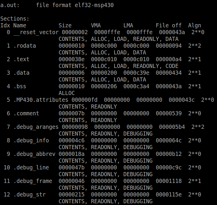
You can see at the top the file format is elf-msp430 – objdump extracts the architecture from the object file. Next is a list of the sections, their name, size, start address (VMA = virtual memory address, LMA = load memory address), the offset of the section in the actual file, the alignment and the section attributes. The __reset_vector, .rodata and .text sections make up the ROM memory region. The .rodata starts at address 0xc000 and the size (16 bytes) is determined by the number and size of read-only variables allocated in the code. The .text section follows directly after at 0xc010. The size of this section is determined by the code size once it is compiled. If the sections that make up a memory region are too big to fit, the linker will throw an error saying there is not enough memory to allocate a section in the memory region. On this device, it is especially easy to run into this with RAM. The RAM region consists of the .data and .bss sections, which start at address 0x200. Since this device has 512 bytes of RAM, the top of RAM is at 0x400 (512 = 0x200; RAM base + RAM size = 0x200 + 0x200 = 0x400). Lets now take a look and locate some of those symbols defined in the linker script. To view the symbols in the object file, use the following command:
/opt/msp430-toolchain/bin/msp430-objdump -t a.out | less
Scroll down or search for the symbol ‘_start’. It should be located at address 0xc010. We know that the .text section should start at 0xc010, and therefore the ‘_start’ symbol is located at this address. Similarly, the first symbol of the .data section is __data_start, which we would expect to be located at address 0x200 – and it is. Another interesting symbol to look at is __romdatastart, which is at 0xc2d4. If you were look at the memory starting at this symbol, it would be the same as __data_start, since the start-up code copies the initialized data from this location to the latter. Finally, the symbol declaring the top of the stack, ‘__stack’, is located at 0x400, as expected. The size of available stack is determined by calculating the difference between the top of stack and the end of the previous section, in this case .noinit. This is easier done using a similar but different utility called ‘nm’, which dumps the symbols from an object file.
nm -n a.out | less
This command puts the symbols in order of their address using the ‘-n’ flag. The last symbol before ‘__stack’ is ‘end’, which marks the end of the .noinit section. Therefore the stack available will be 0x400 – 0x216 = 0x1EA = 490 bytes.
Remember all these symbols and addresses can be changed by modifying the linker script. If you were going to write your own start-up code, you may decide to change some of these. The sections we discussed are the minimum required (or at least generally accepted), but you can add new sections for your own purposes. Hopefully this is all coming together for you, and once you have a grasp of these concepts it becomes much clearer what is happening with your code. It can help you create better quality code by knowing how and where to allocate memory, and how to design your program. You may often be put in a situation to make a decision whether to code for optimal speed or memory. You can’t always have both, and often memory is limited, so you have to compromise accordingly.
The start-up code
Throughout the lesson we have been learning about the start-up code leading up to to the main function. Lets use objdump to examine this code in detail.
/opt/msp430-toolchain/bin/msp430-objdump -S a.out | less
This command uses the ‘-S’ switch to tell objdump to dump the source code mixed with the disassembly (assembly version of your source code). Disassembly only applies to the .text section of the object file, since it is the section that contains the code. The first symbol we see is – big surprise – ‘_start’. The first thing that start does it moves the value of ‘__stack’ (1024 = 0x400) to the stack pointer, R1. The ‘#’ before the symbol means it is moved as an immediate value – i.e. its not loaded from a register, as the value is stored directly in the instruction. Next the watchdog is disabled (which we do again in our code). Then comes the first label (not necessarily a function) ‘__crt0_init_bss’. Side note: assembly is read sequentially through labels – i.e. if there is no branch instruction, the next instruction is loaded regardless of whether it is part of another label. A label could represent a C function, in which case it would be branched to and have a “RET’ instruction at the end. But if written in assembly as some of the start-up code is, it doesn’t have to. Crt0 is the generic name of the start-up code and stands for C run-time. If you have ever tried to compile code and got a linker error saying that the symbol _start cannot be found, you’re likely to be missing crt0.o.
The code following this label does three things, moves __bssstart to R12, clears R13, and then moves __bsssize to R14. Then memset is called. Since the prototype for memset is
int memset(void *ptr, int fill, size_t nbytes)
we can deduce that the following was called
memset(__bssstart, 0, __bsssize);
In other words, this clears the .bss section, as the function name indicates. Next we have the label __crt0_movedata. The symbol __datastart is moved to r13, __romdatastart is moved into r13 and __romdatacopysize is moved into r14. Then memmove is called, so the C implementation would be:
memmove(__datastart, __romdatastart, __romdatacopysize);
which will copy the .data section from flash to RAM so that it can be accessed and modified as required. Next __msp430_init is called, which sets up some C++ exception handlers and may perform some initialization of the standard C library. Finally, R12 is cleared and then our main function is called. Pretty simple, but imperative for code to ever run.
Debugging with mspdebug
Now we are going to actually see all that we learned today in action. First lets take a look at the modifications to our code. I want you to be able to see what passing an argument and a stack backtrace looks like so there a new function called _calculate_checksum which will take two arguments – a pointer to the data and the length of the data in bytes – and return the checksum. The body will be essentially the same as the existing _verify_checksum function.
static uint16_t _calculate_checksum(uint16_t *data, size_t len)
{
    uint16_t crc = 0;
    len = len / 2;

    while (len-- > 0) {
        crc ^= *(data++);
    }

    return crc;
}
Now the _verify_checksum function is stripped down to simply call _calculate_checksum with the correct parameters, and add the result to the value of TLV_CHECKSUM tag and return the result.
static int _verify_cal_data(void)
{
    return (TLV_CHECKSUM + _calculate_checksum((uint16_t *) 0x10c2, 62));
}
What would you expect the compiled code to look do in terms of registers in order to call _calculate_checksum? In the _verify_checksum function, the address of the data needs to be loaded into register R12, and the length of the data into R13. Then the CALL instruction would be used to branch to _calcualate_checksum. When the function returns, the return value will be loaded into R12, and the RET instruction will be called.
Now lets take a look at what happens in main using mspdebug on our launchpad. Program a.out to the device, and set a breakpoint at main using the following command:
setbreak 0xc12a
where 0xc12a is the address of main. Using the old msp430-gdb (before TI took it over), mspdebug used to be able to parse the symbol table and you could tell it to break on a symbol, but somehow that broke. I am looking into it, but no guarantees. Now run the code. The program will run until the main function is called and then stop. When mspdebug hits a breakpoint, it prints out the registers. Lets take a look at these.
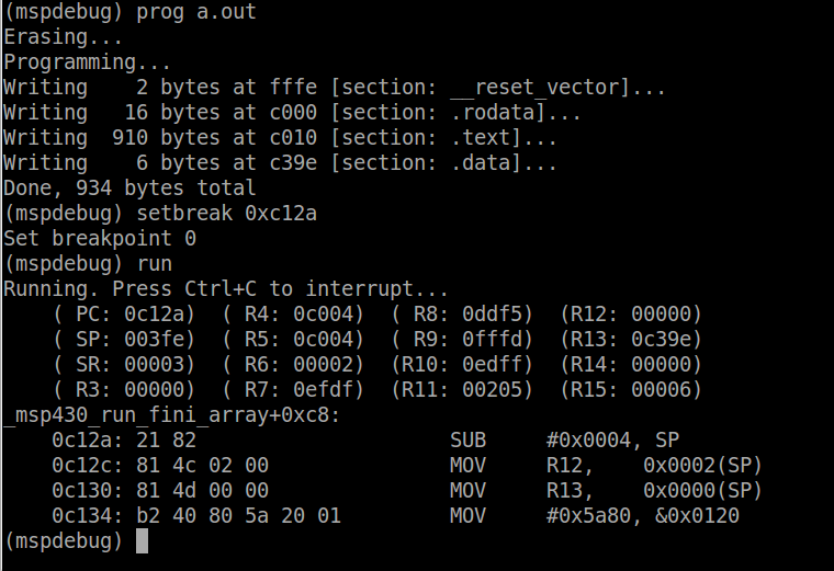
The program counter (PC) is set to 0xc12a as expected, since we told it to break at this address. The stack pointer (SP) is set to 0x3fe, because as we learned earlier, when a function is called, the address of the next instruction is placed on the stack. R12 is set to zero which can be confirmed by the disassembled start-up code we looked at earlier. Now we want to see our new _verify_cal_data function so lets add another breakpoint:
setbreak 0xc1f6
and run again. In the disassembled code provided by mspdebug, we can see that the next two instructions will load the address of the TLV section into R12 and the size into R13 and then call whatever function is at 0xc20a, which is _calculate_checksum. Set one more breakpoint at this address, however, in order to do so we must remove one breakpoint since mspdebug supports up to 2 breakpoints. We can delete the first breakpoint (at main) by using the following command
delbreak 0
where 0 is the index of the breakpoint. Now run one more time. We can see that registers R12 and R13 are set as expected, and the stack pointer is 0x3f6. Now lets try unwinding the stack. To view the memory at the stack pointer, use the md command:
md 0x3f6
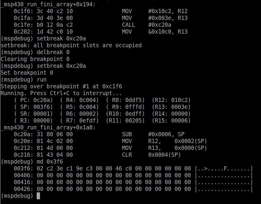
Now, there is an important concept here that needs to be addressed in order to read the memory: endianness. Endianness is the order of bits or bytes in the device. When programming in C the order is standardized (most significant byte and bit on the left) so that it is not architecture dependent and it is the responsibility of the compiler to place the data in the correct ordering. There are several types of endianness and I suggest you read through this if you are not familiar with the concept and ask questions because if you do not understand you will have a very hard time debugging. The MSP430 is a little byte-endian device (see section 2.3 of the MSP430 ABI for more details). This means that if the first byte in the memory dump is actually the least significant byte and the next byte is the most significant byte if storing a standard 16-bit word, as the stack pointer does. If you are storing only a byte, endianness does not apply. So in this case, we can see the first two bytes are 0x02, 0xc2, meaning that the value written to the stack was actually 0xc202. If you look back up to when we broke at _verify_cal_data, this is the address of the next instruction once the current function returns.The next two bytes are also an address, 0xc13e which, if you look at the main function using objdump, is the address of the instruction after calling the _verify_cal_data function. This is very simple example of how to unwind the stack. When you have variables declared in the function, they will be in the stack trace as well. For example _calculate_checksum allocated the variable crc on the stack. To see this variable, we can step through the code using the step command
step
Repeat the command 4 times so that we have executed up to the CLR instruction.

The stack pointer is now at 0x3f0 (notice the first instruction was to subtract 6 from the stack pointer). The arguments of the function are stored on the stack, as well as the crc counter which is then cleared. The compiler chooses in what order to push the variables onto the stack. Finally, if we delete all the breakpoints and set a new one at 0xc202, when the function returns, we can see this:
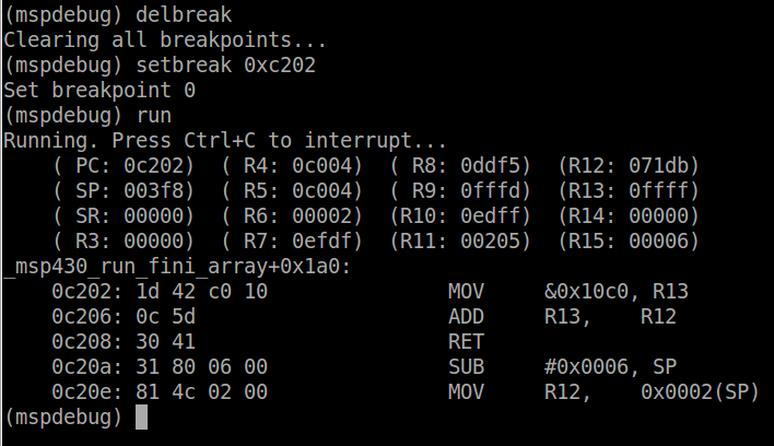
If you look at out code, the _verify_cal_data function takes the return value from _calculate_checksum, and adds its to the TLV checksum. We can see that the value returned using R12 is 0x71db. The value from the address 0x10c0 (the TLV checksum) is loaded into R13, and then added to R12. Since the result is stored in R12, and the RET instruction is called next, the _verify_checksum will return sum of these to values, which we learned last lesson, should be zero if the data is valid.
This lesson really only scraps the surface of these concepts, but it enough to get us started. In the next lesson, we will learn about interrupts, and use the concepts from this lesson to help explain how they work and how they are implemented. We will use interrupts to detect our push button press, and modify the code to
Fantastic lesson, in great detail. Thanks!
Thank you – appreciate the feedback!
This is very good indeed for somebody like me who has always glossed over the details about linker/memory mapping. Btw the word is “onus” not “owness”.
Thanks! As you can see all this programming has taken a toll on my English skills. Sometimes I find myself ending sentences with semicolons :-/
Lots of interesting information 🙂 Regarding the linker scripts, thanks for the explanation. It’s good to know what they are doing even if they are mostly left alone. It was also interesting to know that the symbols defined with the scripts can be referenced within C code! The linked ABI document took a lot of the mystery out of what the compiler is doing in the background. I will definitely take a closer look into it in the future.
One unusual thing that I noticed, you said:
“.data: where initialized read/write data is stored, for example a globally defined variable with an *non-zero* initialized value i.e. int foo = 10;”
I have also heard this before in the past and tried testing it. In the main.c I first added:
unsigned char myValue;
-> the .bss increased in size (two bytes)
Then I assigned an initial value:
unsigned char myValue = 0;
-> the .bss was the original size, the .data increased in size (two bytes)
So, it looks like the compiler puts all initialized values into the .data section regardless of the value assigned. Do you agree?
Hi Joel,
You bring up a very good point. In the MSPGCC, it seems that even if a variable is initialized to zero, it is still placed in the data section. This is interesting because if I do the same test just using regular gcc for x86, it puts anything initialized to zero in the bss (which is what I would expect). I will go and ask on the TI forums if there is a reason for this or if it is a bug in the compiler. At first glance I would think that it would be more efficient to put it in the bss section because then it wouldn’t take up flash aimlessly, but maybe there is some reason. I will add a note in the lesson to mention your point because it can confuse people. Great job at being super diligent going through the material! 🙂
Just realized something I missed, its documented in the ABI that the .bss is only uninitialized variables and the .data section is initialized variables. Still don’t see the reasoning, so I will still ask TI.
Awesome article! Even though I know MSP430 fair bit and have worked on it since 2011, I got new knowledge from this! Great!
Thanks! There’s always something new to learn 🙂 Great to hear that these tutorials are useful for someone with experience in embedded development as well!
The call instruction of the MSP 430 family is a true instruction in the architecture while the ret is indeed emulated, but with a single instruction, move @sp++,pc . It’s a pretty interesting addressing mode, slick.